In reinforcement-learning (RL) post-training for large language models (LLMs), it is common to treat the training set as a flat collection of problems. At each step, a batch of prompts is drawn uniformly, several responses are generated per prompt, rewards are computed, and an algorithm such as GRPO or PPO is applied.
This uniform schedule is convenient, but it ignores a well-known observation from deep RL that some training examples are substantially more informative than others. In value-based RL on Atari, Prioritized Experience Replay (PER) replaces uniform sampling from the replay buffer with sampling biased toward transitions with large temporal-difference (TD) error (Schaul et al. 2016). When integrated into DQN, the median normalized score increased from $48\%$ under uniform sampling to $106\%$ under prioritized sampling, with improvements in $41$ out of $49$ games. Moreover, PER remains one of the most influential components in later agents such as Rainbow (Hessel et al. 2018).
Despite its success, extending this idea directly to RL post-training for LLMs is not straightforward. Unlike value-based RL settings such as Atari, there is no replay buffer of state–action transitions and no TD error defined at the token level. The environment consists of reasoning problems or task simulators; the agent generates complete rollouts; and algorithms such as GRPO operate on groups of responses for a single problem. In this setting, transition-level prioritization is no longer appropriate. Instead, priority has to be defined at the problem level. Recent work has also explored difficulty-aware sampling and rollout reuse in GRPO-style training (Sun et al. 2025). Here, we focus on a simple, non-parametric replay formulation that builds directly on the structure of the GRPO update.
Core method
The goal is to identify, at each training iteration, the subset of problems that are expected to provide the strongest gradient signal under the GRPO update rule. To motivate the construction, we first formalize the per-problem advantage structure and derive a scalar quantity that measures the informativeness of a problem at the current model state.
Consider a fixed problem and assume that we generate $N$ independent responses. Each response receives a binary reward $r_i \in \{0,1\}$, where $r_i = 1$ indicates a correct solution. Let $$ p = \frac{1}{N}\sum_{i=1}^N r_i $$ denote the empirical success rate for this problem in the group of size $N$. GRPO defines the group advantage for response $i$ as $$ A_i = r_i - p. $$
A basic property of this definition is that advantages sum to zero, $$ \sum_{i=1}^N A_i = \sum_{i=1}^N (r_i - p) = \sum_{i=1}^N r_i - Np = Np - Np = 0. $$
Thus the GRPO update extracts information purely from the variation within the set of rewards generated for a single problem. If all $r_i$ are identical (if the model always succeeds or always fails on this problem), then each $A_i$ is zero and the problem yields no gradient signal. Conversely, if the model is correct on some responses and incorrect on others, the advantages take nonzero values and a useful learning signal is produced. Dividing $A_i$ by the standard deviation preserves its zero-sum property and merely scales the resultant gradient magnitude.
To quantify this variation, we consider the mean squared advantage $$ \frac{1}{N}\sum_{i=1}^N A_i^2 = \frac{1}{N}\left(Np(1-p)^2 + N(1-p)p^2\right) = p(1-p). $$
This quantity is the variance of a Bernoulli random variable with mean $p$ and reaches its maximum at $p = \tfrac{1}{2}$. It vanishes at $p=0$ and $p=1$, matching the intuition that a problem the model always solves or always fails provides no contrastive signal for GRPO. We therefore define the priority score of a problem as $$ \omega = p(1-p). $$
Problems with success rates near one-half receive high priority, whereas those with extreme success rates receive low priority. Because $\omega\in[0,1/4]$, the priority score is naturally bounded and comparable across problems. This perspective aligns with broader difficulty-aware views (Sun et al. 2025) that emphasize mid-difficulty examples as especially informative; the contribution here is to make that idea fully explicit in GRPO's group-advantage algebra and to turn it into a concrete replay policy.
At the beginning of training, no empirical estimate of $p$ is available for any problem. Pre-estimating $p$ through multiple rollouts is computationally wasteful for large datasets, and the estimate can instead be obtained on-line as training progresses. To guarantee that every problem is sampled at least once, all priority scores may be initialized to $+\infty$. After a problem has been sampled, its priority score is updated to the finite value $\omega = p(1-p)$ computed from the observed responses. To reduce noise across iterations, $p$ may optionally be maintained using an exponential moving average.
As a more efficient alternative, priority scores can be initialized to any value below $0.25$, the maximum of $p(1-p)$. This initialization allows the algorithm to immediately exploit genuinely high-priority problems as soon as they are identified, without requiring a complete sweep of the dataset. However, this choice no longer guarantees that every problem is forcefully visited at least once. Note also that choosing an initialization value below $0.25$ controls the trade-off between uniform first-time sampling and early exploitation of problems whose priorities exceed that threshold. For example, for a group size of $N=8$, initializing priorities at $0.2$ allows problems with $3$, $4$, or $5$ correct responses to take precedence, while previously unseen problems will not be sampled until later model updates reduce the priorities of the currently dominant problems below $0.2$ (corresponding to correctness levels outside the $3$–$5$ range).
Computational deployment
To efficiently obtain, at each iteration, the $C$ problems with the largest priority scores, we employ a binary max-heap, following Schaul et al. 2016. A binary heap is an array-based representation of a complete binary tree satisfying the heap property that for each index $i$, the parent has priority score no smaller than its children. If indices start at zero, the children of position $i$ reside at positions $2i+1$ and $2i+2$. The maximal-priority element is always stored at index $0$.
The operations extract_max and insert both require $O(\log M)$ time for a heap of size $M$, and are implemented using the standard sift-down and sift-up procedures, which move an element downward or upward until the heap property is restored.
The training iteration proceeds as follows:
- Use extract_max repeatedly to obtain the $C$ problems with the highest current priority scores. These are removed from the heap.
- For each extracted problem, generate $N$ responses, compute their binary rewards, and apply the GRPO update to the model.
- For each such problem, compute a new priority score $\omega = p(1-p)$, where $p$ is the empirical (or exponentially averaged) success rate.
- Reinsert each problem into the heap using insert together with its newly computed priority score.
Because a problem’s priority score is always updated immediately after extraction (never while the problem is still located within the heap) no random deletion or in-place priority modification is required. Consequently, the heap implementation does not need to maintain auxiliary index maps from problem identifiers to heap positions, and its memory footprint consists only of the priority score and the heap arrays. We later discuss exploration, which essentially requires random deletion. Nevertheless, the additional memory need remains negligible even for large $M$.
Important considerations
Forgetting and starvation
Two additional refinements of the priority mechanism address both fully solved and currently unsolvable problems. A problem for which the model achieves $p=1$ consistently yields $\omega=0$ and therefore provides no learning signal. Rather than reinserting such problems into the priority heap, it is useful to maintain a separate pool of fully solved problems. During normal training these problems are ignored, but at a low frequency one may draw a small random batch from this pool and regenerate rollouts. If a problem in this batch remains fully solved, no gradient update is performed; if the model begins to fail on it, then its new empirical success rate determines a positive priority score, and the problem is reinserted into the main heap. This mechanism helps guard against regression on previously mastered material and can reduce the risk of forgetting.
A symmetric consideration applies to problems that currently appear unsolvable. Such problems exhibit $p=0$ and hence also $\omega=0$, which places them permanently at the bottom of the max-heap and effectively prevents them from being revisited. To avoid this starvation effect, these problems may similarly be removed from the heap and stored in an unsolved pool. Periodically, a random subset of this pool can be tested again. If a problem still yields $p=0$, it remains in the unsolved pool; if the model succeeds on at least some responses, that problem receives a positive priority score and is reintroduced into the heap, making it eligible for regular prioritized training. In practice, small tolerance bands such as $p \le \varepsilon$ or $p \ge 1-\varepsilon$ can be used instead of exact zero or one to account for estimation noise.
Both the solved and unsolved pools can be efficiently organized as independent min-heaps keyed by the timestamp of their most recent evaluation. This setup ensures that problems that have been checked most recently are selected again only after all others have been revisited.
Exploration
A further modification introduces controlled exploration directly within the priority heap. Instead of always selecting the problems with the highest priority scores, one may occasionally sample a problem uniformly at random from the heap and temporarily remove it. This requires support for arbitrary deletion, which in turn increases the memory footprint by maintaining a mapping between problem identifiers and their heap positions. Such exploration can prevent the training loop from focusing too narrowly on a small subset of problems whose priority scores fluctuate around intermediate values, and may help the model discover informative problems that would otherwise remain at consistently low priority.
Alternatively, one may replace deterministic max-priority extraction with a stochastic scheme based on a sum-tree structure that supports priority-proportional sampling. In this setup, the probability of selecting a problem is proportional to its current priority score $\omega$, providing a balance between exploitation and exploration. Additional parameters may also be introduced to tune this trade-off. Whether deterministic extraction of the highest-priority problems or stochastic sampling proportional to their priority yields better empirical performance depends on the characteristics of the task distribution and remains an open design choice.
It is also worth emphasizing that, in practice, the dominant computational cost of the environment procedure arises from generating and evaluating model rollouts. These operations are orders of magnitude more expensive than any of the priority-management mechanisms described above. As a consequence, the choice between a deterministic max-heap, an exploration-enhanced heap with arbitrary deletions, or a sum-tree supporting priority-proportional sampling should be driven primarily by empirical training dynamics rather than computational considerations.
Learning rate
The use of prioritized replay directly amplifies the magnitude of the learning signal. Because prioritized sampling favors problems with high advantage variance, the expected per-update advantage under prioritized GRPO is larger than it would be under uniform sampling. Since the policy-gradient loss scales linearly with advantage, this amplification translates into larger effective gradients during optimization.
A practical implication is that learning rates tuned for standard GRPO may become overly aggressive when used with prioritized replay. Without adjustment, the interaction between higher gradient magnitudes and unchanged hyperparameters can increase training instability. In small-scale experiments, this effect appears when applying off-the-shelf configurations commonly used in frameworks such as verl. In practice, it may therefore be necessary to reduce the base learning rate or apply adaptive learning-rate schedules when enabling prioritized sampling. More generally, hyperparameters that implicitly depend on gradient scale, such as clipping ranges, entropy coefficients, or EMA smoothing constants, may also require retuning to ensure stable training dynamics under prioritized replay.
Concise reasoning
Concise reasoning has recently become a central objective in the development of reasoning-oriented language models. The term refers to achieving high problem-solving performance while producing substantially fewer tokens. Fatemi et al. (2025) showed that continued training on correct responses causes the optimization dynamics to favor shorter and more direct solutions, whereas reinforcement on incorrect responses tends to produce unnecessarily verbose outputs. This effect arises solely from the structure of the loss and the advantage sign, independent of any explicit incentive toward brevity.
Motivated by this phenomenon, it can be desirable to introduce a slight bias toward problems on which the model already performs relatively well. In the core method described above, the priority score $\omega = p(1-p)$ is perfectly symmetric around $p = 1/2$. For example, in a group of $N=8$, a problem with $k=6$ correct responses ($p=0.75$) receives the same priority score as a problem with $k=2$ correct responses ($p=0.25$), since both yield $\omega = \tfrac{6}{8}\cdot\tfrac{2}{8} = 0.1875$. However, if concise reasoning is desired as a secondary objective, it may be preferable to prioritize the former problem to reinforce rollouts with a higher rate of correct answers.
There are several ways to introduce this bias without fundamentally altering the prioritization mechanism. One simple approach is to add a small positive constant to the priority score whenever $k \geq N/2$. This preserves the maximum at $p=1/2$ while breaking the symmetry between $p$ and $1-p$ in a controlled manner. The constant can be set sufficiently small so that it merely breaks ties between symmetric cases of $k$ and $N-k$ without affecting the ranking of other pairs. This lightweight adjustment nudges the prioritized replay process toward promoting concise reasoning while retaining the core benefits of the variance-based priority measure.
Experiments
Our empirical evaluation is intentionally limited by compute budget and should be interpreted as a proof of concept rather than a comprehensive study. The goal is to assess the behavior of prioritized replay in a realistic but constrained training setting, rather than to perform large-scale hyperparameter optimization.
We fine-tune Qwen2.5-7B using GRPO on a stratified subset of 1,000 problems from the GURU dataset (Cheng et al. 2025). GURU contains 54K math problems with different levels of difficulty and reports two success rates $p_{guru}$ for each problem, estimated using 64 samples from two models: Qwen2.5-7B and the stronger Qwen3-30B. The dataset additionally applies several filtering steps, including the removal of duplicates and problems that achieve $p_{guru}=0.0$ on Qwen3-30B. Related math reasoning datasets such as DeepSeekMath (Shao et al. 2024) follow a similar philosophy of building challenging benchmarks from model-derived signals.
From the original set of 54,404 math problems, we select a smaller subset of 47,844 problems with $p_{guru}>0.5$ on Qwen3-30B. This selection yields problems that are reasonably learnable under our smaller-scale training regime. Despite this filtering, the subset still contains a large fraction of fully or nearly unsolvable problems for Qwen2.5-7B (over $60\%$). Finally, for our experiments, we select a random subset of 1,000 problems, stratified to match the difficulty distribution of the full dataset. The labels $p_{guru}$ are not used for initialization or training.
For each training step, we sample a batch of $4$ problems and generate $8$ rollouts per problem at temperature $0.7$, yielding $32$ response–reward pairs per step. We use $A_i = r_i - p$ without standard-deviation normalization, where $p$ is the group mean reward. The reward function assigns binary scores based on answer correctness, using the Qwen Math Eval Toolkit (Yang et al., 2025) for robust symbolic equivalence checking. For the codebase, we fork from verl and add the prioritized replay mechanism on top of it.
Success rates are tracked using exponential moving average with $\alpha = 0.8$. Problems are prioritized by $\omega = \bar{p}(1-\bar{p}) + \epsilon$, where $\bar{p}$ is the EMA success rate and $\epsilon=10^{-4}$ is a small bias when $p\ge 0.5$. All problems are initialized at $\omega=0.2$. As training advances, problems with $p = 1$ (fully solved) or $p = 0$ (fully unsolved) are moved to separate pools and periodically retested (every $10$ steps, $1$ from the solved pool and $3$ from the unsolved pool). Exploration is performed at the batch level: $12.5\%$ of training batches are sampled uniformly at random from the main heap rather than by priority. The baseline uses identical hyperparameters but with uniform random sampling instead of prioritized sampling.
Models are evaluated every $25$ training steps on the MATH-500 benchmark ($500$ problems) and AIME-2024 ($30$ problems), using $4$ rollouts per problem at temperature $0.7$. We use AdamW with learning rate $10^{-6}$, no weight decay, no learning rate schedule, and no KL penalty. PPO clipping ratio is $0.2$ with gradient clipping at $1.0$. Training runs for $250$ steps on 8×B200 GPUs. Note that with $250$ training steps and $4$ problems per step, the baseline setting covers the entire dataset once, whereas prioritized sampling will only expose the model to a subset of it.
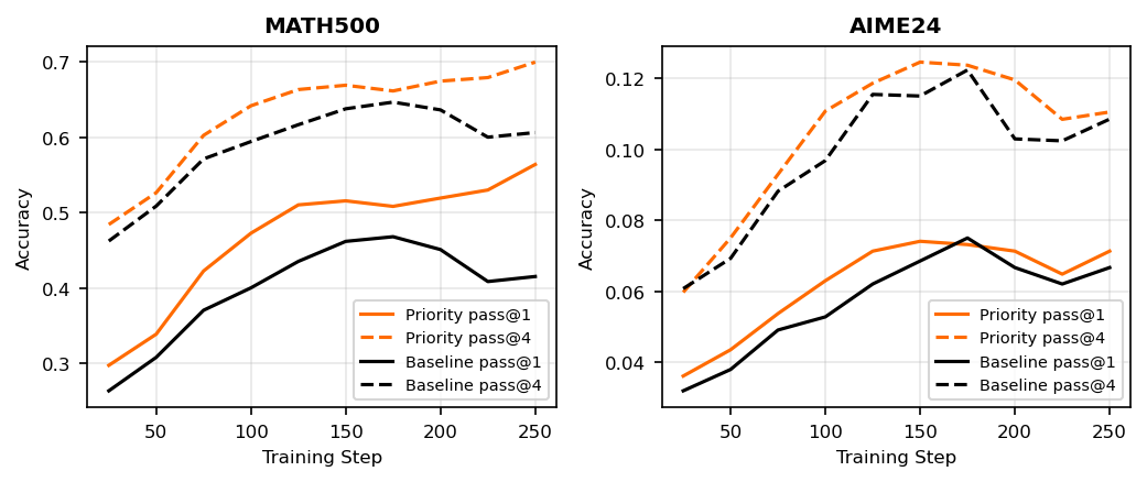
Figure 1 presents pass@1 and pass@4 performance of the uniform baseline and the prioritized sampling method, with curves smoothed using a window of three prior values. Within the reported 250 steps, the prioritized sampler almost always outperforms uniform sampling on both benchmarks and for both pass@1 and pass@4.
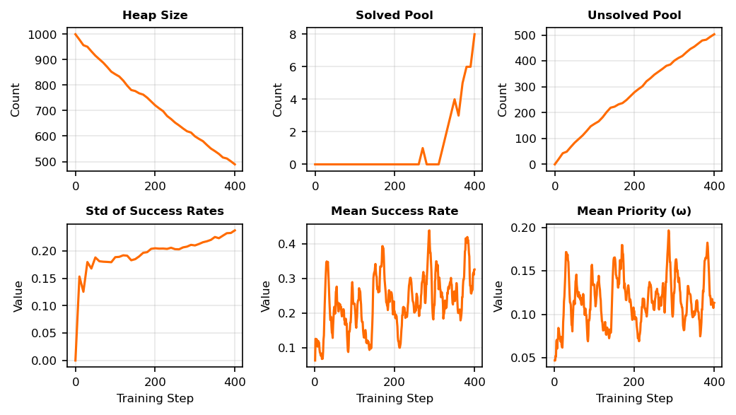
Figure 2, Row 1. The heap size denotes the number of learnable problems, which are those with intermediate success rates $0 < p < 1$ that produce meaningful gradients. As training progresses, problems gradually migrate to the solved pool ($p = 1$) or the unsolved pool ($p = 0$). A healthy training trajectory is characterized by a steady flow from the heap into these pools as the model's competence boundaries become more clearly defined. In our small scale experiment with only $250$ training steps, none of the problems reached full success and therefore none entered the solved pool, while many problems were progressively classified as unsolvable. We also observe that more than $600$ problems remain unseen during this run, because the initialization strategy prioritizes problems with $3$–$5$ correct answers, when such problems are available, instead of unseen problems. This sampling bias may also help explain the behavior observed beyond step $250$ in our briefly extended but incomplete runs, where performance oscillates without substantial improvement. Limitted exposure to unseen data and potentially the use of a large learning rate may be contributing factors that require further investigation.
Figure 2, Row 2. The standard deviation of success rates reflects the diversity of problem difficulty as perceived by the model. High values (approximately $0.4$ to $0.5$) indicate a wide spread of difficulties, with some problems being easy (high $p$), some hard (low $p$), and others in between. This situation is generally desirable for prioritized sampling, because it allows the sampler to meaningfully distinguish among problems. In contrast, a low standard deviation indicates that most problems have similar success rates, which may occur when problems are uniformly easy ($p \approx 1$), uniformly hard ($p \approx 0$), or clustered around an intermediate difficulty level.
In this experiment, the std of success rates remains relatively small throughout training, which is consistent with the fact that all problems are initialized with equal success estimates and many problems remain unseen within the $250$ training steps. However, the observation that the standard deviation stabilizes near $0.2$ suggests limited exploration of unseen data. The plot indicates that, in the last $60$ steps of training, the active portion of the heap is dominated by a set of solvable problems whose priorities remain higher than the default priority assigned to unseen problems. As a result, although unseen problems are still present in the heap, they are rarely selected for training. At the same time, the $12.5\%$ mechanical exploration does not appear to compensate for this effect. This is likely because a substantial fraction of the dataset is truly unsolvable and small exploration tends to add additional problems to the unsolved pool rather than enriching the set of learnable problems, which is also reflected in the steadily (nearly linear) increasing number of items classified as unsolved.
Discussion
This work presents a problem-level formulation of prioritized replay for RL post-training and shows that the method can be integrated into a realistic training pipeline. In the experiments described above, prioritized sampling provides stronger early-stage performance than uniform sampling on both MATH-500 and AIME-2024 for pass@1 and pass@4 under the same configuration that is commonly used with uniform sampling.
These results should be viewed as an initial proof of concept rather than a comprehensive evaluation. The compute budget limited the range of configurations we could explore and constrained training to a relatively small number of steps. A systematic examination of configuration choices, particularly learning rates, exploration schedules, and the management of solved and unsolved pools, remains future work.
From a conceptual perspective, problem-level prioritized replay provides a model-driven complement to curriculum learning and to more complex difficulty-prediction and rollout-replay methods. Classical curricula and recent LLM curricula organize tasks into difficulty tiers and design schedules that move from easy to hard (Bengio et al. 2009; Narvekar et al. 2020). This requires predefined difficulty labels or an auxiliary policy, and the resulting notion of difficulty may not match the behavior of the particular base model under training. In contrast, the priority score $\omega = p(1-p)$ is computed directly from the model’s current performance on each problem. It requires no labels, adapts automatically as the model improves, and focuses training on the boundary between problems the model has mastered and problems that remain out of reach.
What practitioners should remember
1. The priority score comes directly from GRPO.
For a fixed problem, the mean squared GRPO advantage equals $p(1-p)$, where $p$ is the empirical success rate. The same quantity serves as a natural problem-level priority score.
2. Problems with intermediate success rates drive learning in GRPO-style methods.
Problems that the model always solves or always fails contribute no gradient signal under GRPO. Prioritized replay allocates more updates to problems the model solves only intermittently.
3. A max-heap is sufficient for scheduling.
A binary max-heap over problem indices, together with solved and unsolved pools and periodic retesting, realizes the prioritization scheme with negligible overhead compared to rollouts.
4. Learning rates need to be revisited.
Prioritization increases typical gradient magnitudes. Learning rates and related hyperparameters tuned under uniform sampling may need to be reduced or otherwise adjusted.
5. Exploration and pool management matter.
A small amount of uniform exploration and explicit handling of solved and unsolved problems are important to avoid overly narrow focus and to mitigate forgetting and starvation.
6. No labels or curricula are required.
The method does not rely on predefined difficulty tiers or curriculum schedules. The effective curriculum emerges from the model’s evolving success rates on individual problems.
7. The method is a drop-in extension of GRPO pipelines.
Prioritized replay operates entirely at the problem-selection level and is compatible with existing GRPO implementations and infrastructure.
References
- T. Schaul, J. Quan, I. Antonoglou, D. Silver (2016). Prioritized Experience Replay. ICLR.
- M. Hessel et al. (2018). Rainbow: Combining Improvements in Deep Reinforcement Learning. AAAI.
- Y. Sun et al. (2025). Improving Data Efficiency for LLM Reinforcement Fine-tuning Through Difficulty-targeted Online Data Selection and Rollout Replay. arXiv:2506.05316.
- Z. Shao et al. (2024). DeepSeekMath: Pushing the Limits of Mathematical Reasoning. arXiv:2402.03300.
- Z. Cheng et al. (2025). Revisiting Reinforcement Learning for LLM Reasoning from A Cross-Domain Perspective. arXiv:2506.14965.
- Y. Bengio et al. (2009). Curriculum Learning. ICML.
- S. Narvekar et al. (2020). Curriculum Learning for Reinforcement Learning Domains: A Framework and Survey. JMLR.
- M. Fatemi, B. Rafiee, M. Tang, K. Talamadupula (2025). Concise Reasoning via Reinforcement Learning.
- Yang et al. (2025). Qwen2 technical report. arXiv:2407.10671.